
Every optical designer has experienced the same heartbreak. You receive a design file showing an MTF curve that hugs the diffraction limit across the entire field. The software predicts pinpoint sharpness. Yet, when the first pilot batch arrives from the machine shop and cleanroom, the images tell a different story.
Corner resolution collapses. Contrast drops at critical spatial frequencies. Lens-to-lens consistency varies wildly across the production line. What looked brilliant in Zemax falls apart on the factory floor.
The problem is rarely the optical formula itself. The failure happens in the translation from pure math to manufactured hardware. In high-precision vision systems, an impressive nominal curve does not guarantee a good MTF lens in mass production.
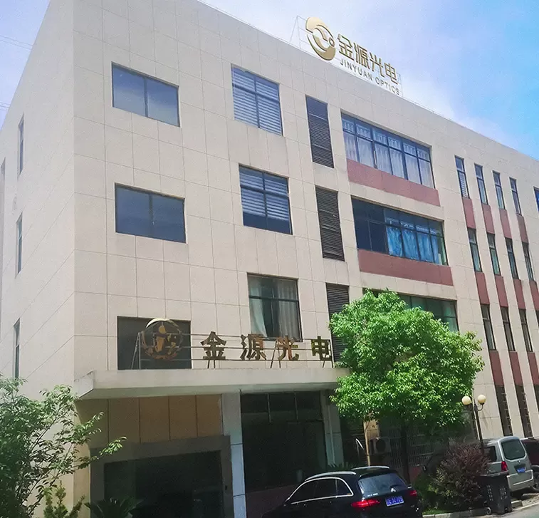
At Jinyuan Optics, we work with system integrators to solve this exact bottleneck. Before locking down your hardware architecture, you need to know how to specify optical performance that survives real-world assembly, thermal swings, and mechanical shock.
Planning a new vision platform? Contact the Jinyuan engineering team to request a complimentary optical tolerance review for your sensor.
The Fallacy of the Nominal MTF Curve
Modulation Transfer Function (MTF) measures how faithfully an optical system transfers contrast from the object to the sensor at specific spatial frequencies. Optical software can easily generate an ideal curve under zero-tolerance conditions. In simulation, every surface is mathematically perfect, every air gap is exact, and alignment never drifts.
Real-world manufacturing breaks these ideal assumptions immediately. Grinding tools introduce figure errors. Glass melts deviate slightly in refractive index. Mechanical barrels have machining tolerances. Assembly technicians introduce microscopic decenters.
A poorly conceived design might show 60% contrast at 100 line pairs per millimeter (lp/mm) on paper. But because its internal elements carry tight radii and hyper-sensitive air spaces, a 5-micron manufacturing shift can degrade that performance by half.
A truly good MTF lens prioritizes as-built yield over theoretical perfection. It features relaxed optical surfaces that tolerate real-world manufacturing limits while holding contrast steady across thousands of units.
Monte Carlo Analysis: Separating Theory from Mass Production
To evaluate whether a design can yield a reliable production lens, optical engineers rely on Monte Carlo tolerancing. Instead of running a single perfect simulation, this method generates hundreds or thousands of randomized builds.
Each virtual build introduces realistic manufacturing errors within predefined statistical bounds:
Surface Curvature and Irregularity: Variations measured in Newton rings or fractions of a wavelength.
Element Thickness and Air Spacing: Axial shifts caused by machining tolerances in spacers and retaining rings.
Decenter and Tilt: Lateral displacement and angular runout of individual elements relative to the mechanical axis.
Material Homogeneity: Slight shifts in index of refraction ($n_d$) and Abbe number ($V_d$) between glass batches.
When reviewing design proposals, look closely at the 90th or 95th percentile Monte Carlo curve. If your nominal contrast sits at 0.5 at your target frequency, but the 90% yield curve plummets to 0.15, the lens will fail in mass production. An experienced manufacturer adjusts element geometries to widen tolerance margins, ensuring predictable optical transfer function performance on the assembly line.
Precision Assembly: Why Active Alignment Changes Everything
Passive optical assembly relies entirely on mechanical stops and barrel tolerances. For legacy sensors with 5-micron pixels, this approach works well enough. However, high-density sensors expose the limits of passive mechanical stacking.
When working with sub-2-micron pixel pitches, mechanical tolerances alone cannot prevent asymmetric aberrations like coma and astigmatism. This is where Active Alignment (AA) becomes necessary.
During active alignment, the lens group—or final corrective element—is manipulated along multiple degrees of freedom (X, Y, Z, tip, and tilt) while the system projects live test patterns onto a target sensor or collimator. Collimated beams project through the optical train, and automated software computes the wavefront distortion in real time.
The system locks the components into position only when the real-time MTF reaches its optimized threshold across all field points. By actively compensating for cumulative manufacturing stack-up, active alignment turns what would have been scrap parts into high-yield, diffraction-limited assemblies.
Matching the Lens MTF to Sensor Physics
A lens does not operate in a vacuum. It works as an integrated pair with an image sensor. Evaluating a good MTF lens requires grounding your spatial frequency targets directly in the physical architecture of that sensor.
Calculating the Nyquist Cutoff
The spatial resolution limit of any digital imaging system is governed by the Nyquist frequency of the sensor. The Nyquist limit ($f_N$) represents the point where two sensor pixels cover exactly one line pair:
$f_N = 1000 / (2 \times \text{Pixel Pitch in }\mu m)$
Consider how modern pixel geometries drive these requirements:
3.45 $\mu m$ Pixel (e.g., Sony Pregius Gen 2): Nyquist frequency is approximately 145 lp/mm.
2.40 $\mu m$ Pixel (e.g., Sony Pregius S Gen 4): Nyquist frequency jumps to 208 lp/mm.
1.40 $\mu m$ Pixel (e.g., High-resolution mobile/embedded CMOS): Nyquist frequency hits 357 lp/mm.
If you pair a 2.4-micron sensor with a lens tested only to 100 lp/mm, you leave half of the sensor's resolving power on the table. Conversely, you do not need 70% contrast at Nyquist. Targeting an MTF between 0.20 and 0.30 at the Nyquist frequency is standard for industrial inspection, preserving detail without introducing excessive aliasing or false color artifacts.
Balancing Center vs. Edge Performance
Many off-the-shelf catalog lenses claim high MTF values, but bury the fine print: that contrast exists only in the center 20% of the image circle. At the field edges, sagittal and tangential MTF lines plunge due to uncorrected field curvature, astigmatism, and lateral color.
In automated optical inspection (AOI), semiconductor metrology, and wide-area logistics sorting, edge resolution matters just as much as on-axis sharpness. Defect detection algorithms demand uniform edge-to-edge contrast.
When Jinyuan customizes an optical assembly, our engineers balance the field curvature profile to flatten the image plane across the full diagonal format. A truly balanced lens may trade 5% of its on-axis contrast to pull the far-corner MTF from 0.10 up to 0.30, providing a uniform baseline for computer vision algorithms.
Environmental Stability: MTF Beyond the Laboratory
A lab bench maintains a comfortable 20°C. Industrial cameras, autonomous mobile robots (AMRs), and aerial mapping pods do not. If your vision system operates outdoors or near high-temperature machinery, thermal drift can ruin your optical performance.
Optical-Mechanical Athermalization
As ambient temperatures shift from -40°C to +85°C, two physical changes occur within an optical assembly:
The refractive index of glass shifts based on its thermal coefficient ($dn/dT$).
The lens elements and mechanical barrels expand or contract based on their Coefficient of Thermal Expansion (CTE).
In an uncompensated lens, the focal plane drifts away from the sensor plane as temperatures swing. High-frequency MTF drops to zero because the system simply falls out of focus.
Passive optical athermalization solves this challenge without bulky heaters or motor-driven actuators. By pairing specific optical glasses with opposing $dn/dT$ values alongside a balanced combination of aluminum, brass, or engineered plastics, the thermal expansion of the barrel cancels out the optical focal shift. The focal point remains fixed on the sensor cover glass across the entire operating range.
Vibration and Shock Immunity
High-G environments like manufacturing stamping lines or automotive perception suites present another threat: mechanical displacement. If an adhesive bond shears or a threaded lock ring backs out by a fraction of a thread, element spacing shifts.
Ruggedized lens designs eliminate moving internal parts. Designers replace variable iris mechanisms with fixed aperture stops and lock all optical elements in place with continuous 360-degree adhesive bonds. This mechanical stability ensures your specified MTF remains intact after thousands of hours of high-frequency vibration.
How to Write an Unambiguous MTF Specification for RFQs
One of the most frequent procurement mistakes is sending an RFQ that states: "The lens must have good image quality with MTF > 0.3." This statement is completely ambiguous. It leaves critical optical parameters open to interpretation, inviting vendors to quote under-engineered designs.
To source a reliable custom lens, define your requirements using explicit, measurable parameters:
Target Spatial Frequencies: Specify exact values (e.g., 70 lp/mm and 140 lp/mm), rather than vague labels.
Field Positions: Define contrast minimums on-axis (0.0F), at mid-field (0.7F), and at the extreme corner (1.0F).
Wavelength Weighting: State your exact working spectral band, whether it is visible (400–700 nm), narrow-band LED (e.g., 850 nm $\pm$ 10 nm), or SWIR (900–1700 nm).
Conjugate Distance / Working Distance: Explicitly state the object-to-lens distance. A lens optimized for infinity will show severe spherical aberration when focused at 200 mm.
Acceptable Astigmatism Delta: Cap the allowable separation between Sagittal (S) and Tangential (T) curves (e.g., $|MTF_s - MTF_t| \le 0.10$).
Verification and Metrology: The Factory Acceptance Test
Never rely on simulation plots as proof of quality. Before accepting production lots, confirm how your supplier verifies finished assemblies.
Tier-one optical manufacturers rely on specialized optical test stations, such as Trioptics ImageMaster® systems, to measure physical transmission MTF. These instruments spin the lens through precise azimuthal angles while off-axis collimators verify contrast at multiple field angles simultaneously.
A legitimate production run should always ship with an MTF Certificate of Conformance (CoC). This document confirms that sampled lenses meet your contractual spatial frequency thresholds across the full format before they leave the factory floor.
Frequently Asked Questions
Q1: Why does my lens produce blurry images even though the MTF curve
shows high values?
A1: This mismatch usually occurs when the lens
was evaluated under conditions that do not match your setup. If the vendor
tested the lens at infinity, but your machine inspects objects at a 300 mm
working distance, uncorrected spherical aberration will degrade contrast.
Mismatched spectral weighting or sensor cover glass thickness can also introduce
significant aberrations.
Q2: What is an acceptable difference between Sagittal and Tangential
MTF?
A2: In high-precision vision systems, you should keep the delta
between Sagittal and Tangential MTF under 0.10 to 0.15 across the working field.
Large splits between these curves indicate uncorrected astigmatism or lateral
color, which makes fine features look stretched, smeared, or double-edged along
radial lines.
Q3: How much contrast (MTF value) does an industrial algorithm need
to detect edges reliably?
A3: Most edge-detection and
feature-extraction algorithms require at least 15% to 20% contrast (an MTF value
of 0.15 to 0.20) at the sensor's Nyquist frequency. While human inspectors
prefer higher contrast for visual comfort, machine vision algorithms can
reliably process down to 0.15, provided the image sensor maintains a clean
signal-to-noise ratio (SNR).
Q4: Why does MTF drop when I stop down the lens aperture too
far?
A4: While stopping down an aperture (e.g., moving from f/2.8 to
f/8) helps eliminate geometric aberrations like coma and spherical error,
stopping down too far (past f/11 or f/16 on modern sensors) causes diffraction
to take over. Airy disks expand, spreading light across adjacent pixels and
setting a hard physical ceiling on the lens resolution.
Q5: Can image processing software compensate for a lens with poor
MTF?
A5: Software deconvolution and sharpening filters can boost
mid-frequency contrast, but they cannot recover spatial frequencies that have
dropped to zero. Sharpening an image from a low-contrast lens amplifies sensor
noise and introduces edge halos. High-reliability systems must resolve critical
frequencies optically before applying digital enhancement.
Build Your Next Optical Platform with Confidence
A high-performance imaging system requires more than theoretical promises on a datasheet. It demands an optical assembly built to maintain its sharpness against thermal expansion, rough mechanical handling, and strict manufacturing tolerances. Knowing the difference between nominal design files and real-world production performance is what keeps your project on schedule and within budget.
At Jinyuan Optics, we specialize in high-yield, custom-engineered optical solutions. We design our assemblies from the ground up to match your exact sensor architecture, operating environment, and mass-production volume requirements.
Ready to validate your optical
specifications?
Submit your sensor model, mechanical envelope, and
target working distance today. Our engineering team will deliver a comprehensive
optical tolerance analysis and a direct feasibility review for your
next-generation vision platform.